02. Neural Network classification with PyTorch
Classification is a problem of predicting whether something is one thing or another (there can be multiple things as the options).
Book version of this notebook - https://www.learnpytorch.io/02_pytorch_classification/ All other resources - https://github.com/mrdbourke/pytorch-deep-learning Ask questions here - https://github.com/mrdbourke/pytorch-deep-learning/discussions
1. Make classification data and get ready
import sklearn
from sklearn.datasets import make_circles

# Make 1000 samples
n_samples = 1000

# Create circles
X, y = make_circles(n_samples,
                    noise=0.03,
                    random_state=42)
len(X), len(y)
(1000, 1000)
print(f"First 5 samples of X:\n {X[:5]}")
print(f"First 5 samples of y:\n {y[:5]}")
First 5 samples of X:
 [[ 0.75424625  0.23148074]
 [-0.75615888  0.15325888]
 [-0.81539193  0.17328203]
 [-0.39373073  0.69288277]
 [ 0.44220765 -0.89672343]]
First 5 samples of y:
 [1 1 1 1 0]
# Make DataFrame of circle data
import pandas as pd
circles = pd.DataFrame({"X1": X[:, 0],
                        "X2": X[:, 1],
                        "label": y})
circles.head(10)
| X1 | X2 | label | |
|---|---|---|---|
| 0 | 0.754246 | 0.231481 | 1 |
| 1 | -0.756159 | 0.153259 | 1 |
| 2 | -0.815392 | 0.173282 | 1 |
| 3 | -0.393731 | 0.692883 | 1 |
| 4 | 0.442208 | -0.896723 | 0 |
| 5 | -0.479646 | 0.676435 | 1 |
| 6 | -0.013648 | 0.803349 | 1 |
| 7 | 0.771513 | 0.147760 | 1 |
| 8 | -0.169322 | -0.793456 | 1 |
| 9 | -0.121486 | 1.021509 | 0 |
circles.label.value_counts()
| count | |
|---|---|
| label | |
| 1 | 500 |
| 0 | 500 |
# Visualize, visualize, visualize
import matplotlib.pyplot as plt
plt.scatter(x=X[:, 0],
            y=X[:, 1],
            c=y,
            cmap=plt.cm.RdYlBu);
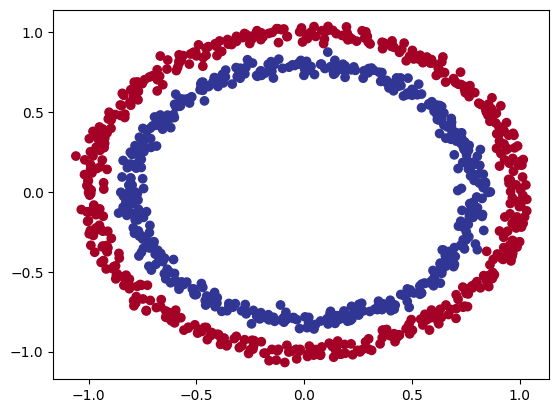
Note: The data we’re working with is often referred to as a toy dataset, a dataset that is small enough to experiment but still sizeable enough to practice the fundamentals.
1.1 Check input and output shapes
X.shape, y.shape
((1000, 2), (1000,))
X
array([[ 0.75424625,  0.23148074],
       [-0.75615888,  0.15325888],
       [-0.81539193,  0.17328203],
       ...,
       [-0.13690036, -0.81001183],
       [ 0.67036156, -0.76750154],
       [ 0.28105665,  0.96382443]])
# View the first example of features and labels
X_sample = X[0]
y_sample = y[0]

print(f"Values for one sample of X: {X_sample} and the same for y: {y_sample}")
print(f"Shapes for one sample of X: {X_sample.shape} and the same for y: {y_sample.shape}")
# Scalars do not have shapes
Values for one sample of X: [0.75424625 0.23148074] and the same for y: 1
Shapes for one sample of X: (2,) and the same for y: ()
1.2 Turn data into tensors and create train and test splits
import torch
torch.__version__
'2.5.1+cu121'
type(X), X.dtype
(numpy.ndarray, dtype('float64'))
# Turn data into tensors
X = torch.from_numpy(X).type(torch.float) # change datatype to float32 (pytorch default)
y = torch.from_numpy(y).type(torch.float)

X[:5], y[:5]
(tensor([[ 0.7542,  0.2315],
         [-0.7562,  0.1533],
         [-0.8154,  0.1733],
         [-0.3937,  0.6929],
         [ 0.4422, -0.8967]]),
 tensor([1., 1., 1., 1., 0.]))
type(X), X.dtype, y.dtype
(torch.Tensor, torch.float32, torch.float32)
# Split data into training and test sets
from sklearn.model_selection import train_test_split

X_train, X_test, y_train, y_test = train_test_split(X,
                                                    y,
                                                    test_size=0.2, # 0.2 = 20% of data will be test & 80% wil be train
                                                    random_state=42)
len(X_train), len(X_test), len(y_train), len(y_test)
(800, 200, 800, 200)
2. Building a model
Let’s build a model to classify our blue and red dots.
To do so, we want to:
- Setup device agnostic code so our code will run on an accelerator (GPU) if there is one
- Construct a model (by subclassing
nn.Module) - Define a loss function and optimizer
- Create a training and test loop
# Import PyTorch and nn
import torch
from torch import nn

# Make device agnostic code
device = "cuda" if torch.cuda.is_available() else "cpu"
device
'cuda'
X_train
tensor([[ 0.6579, -0.4651],
        [ 0.6319, -0.7347],
        [-1.0086, -0.1240],
        ...,
        [ 0.0157, -1.0300],
        [ 1.0110,  0.1680],
        [ 0.5578, -0.5709]])
Now we’ve setup device agnostic code, let’s create a model that:
- Subclasses
nn.Module(almost all models in PyTorch subclassnn.Module) - Create 2
nn.Linear()layers that are capable of handling the shapes of our data - Defines a
forward()method that outlines the forward pass (or forward computation) of the model - Instantiate an instance of our model class and send it to the target
device
X_train.shape
torch.Size([800, 2])
y_train[:5]
tensor([1., 0., 0., 0., 1.])
from sklearn import datasets
# 1. Construct a model that subclasses nn.Module
class CircleModelV0(nn.Module):
  def __init__(self):
    super().__init__()
    # 2. Create 2 nn.Linear layers capable of handling the shapes of our data
    self.layer_1 = nn.Linear(in_features=2, out_features=5) # takes in 2 features and upscales to 5 features
    self.layer_2 = nn.Linear(in_features=5, out_features=1) # takes in 5 features from previous layer and outputs a single feature (same shape as y)

    #self.two_linear_layers = nn.Sequential(
    #    nn.Linear(in_features=2, out_features=5),
    #    nn.Linear(in_features=5, out_features=1)
    #)

  # 3. Definde a forward() method that outlines the forward pass
  def forward(self, x):
    return self.layer_2(self.layer_1(x)) # x -> layer 1 -> layer 2 -> output
    #return two_linear_layers(x)

# 4. Instantiate an instance of our model class and send it to the target device
model_0 = CircleModelV0().to(device)
model_0
CircleModelV0(
  (layer_1): Linear(in_features=2, out_features=5, bias=True)
  (layer_2): Linear(in_features=5, out_features=1, bias=True)
)
device
'cuda'
next(model_0.parameters()).device
device(type='cuda', index=0)
# Let's replicate the model above using nn.Sequential(), same as commented code above
model_0 = nn.Sequential(
    nn.Linear(in_features=2, out_features=5),
    nn.Linear(in_features=5, out_features=1)
).to(device)

model_0
Sequential(
  (0): Linear(in_features=2, out_features=5, bias=True)
  (1): Linear(in_features=5, out_features=1, bias=True)
)
model_0.state_dict()
OrderedDict([('0.weight',
              tensor([[ 0.5763, -0.5214],
                      [-0.1052, -0.5952],
                      [ 0.4719,  0.0889],
                      [-0.2932, -0.2321],
                      [-0.0147, -0.6714]], device='cuda:0')),
             ('0.bias',
              tensor([-0.2953,  0.3209,  0.3331,  0.6216, -0.1047], device='cuda:0')),
             ('1.weight',
              tensor([[ 0.2756,  0.2582, -0.2747,  0.0817, -0.3515]], device='cuda:0')),
             ('1.bias', tensor([0.0958], device='cuda:0'))])
# Make predictions
with torch.inference_mode():
  untrained_preds = model_0(X_test.to(device))
print(f"Length of predictions: {len(untrained_preds)}, Shape: {untrained_preds.shape}")
print(f"Lenght of test samples: {len(X_test)}, Shape: {X_test.shape}")
print(f"\nFirst 10 predictions:\n{torch.round(untrained_preds[:10])}")
print(f"\nFirst 10 labels:\n{y_test[:10]}")
Length of predictions: 200, Shape: torch.Size([200, 1])
Lenght of test samples: 200, Shape: torch.Size([200, 2])

First 10 predictions:
tensor([[0.],
        [-0.],
        [0.],
        [-0.],
        [0.],
        [0.],
        [0.],
        [0.],
        [0.],
        [-0.]], device='cuda:0')

First 10 labels:
tensor([1., 0., 1., 0., 1., 1., 0., 0., 1., 0.])
X_test[:10], y_test[:10]
(tensor([[-0.3752,  0.6827],
         [ 0.0154,  0.9600],
         [-0.7028, -0.3147],
         [-0.2853,  0.9664],
         [ 0.4024, -0.7438],
         [ 0.6323, -0.5711],
         [ 0.8561,  0.5499],
         [ 1.0034,  0.1903],
         [-0.7489, -0.2951],
         [ 0.0538,  0.9739]]),
 tensor([1., 0., 1., 0., 1., 1., 0., 0., 1., 0.]))
2.1 Setup loss function and optimizer
Which loss function or optimizer should you use?
Again… this is problem specific.
For example for regression you might want MAE or MSE (mean absolute error or mean squared error).
For classification you might want binary cross entropy or categorical cross entropy (cross entropy).
As a reminder, the loss function measures how wrong your models predictions are.
And for optimizers, two of the most common and useful are SGD and Adam, however PyTorch has many build-in options.
- For some common choices of loss functions and optimizers - https://www.learnpytorch.io/02_pytorch_classification/#21-setup-loss-function-and-optimizer
- For the loss function, we’re going to use
torch.nn.BECWithLogitsLoss(), for more on what binary cross entropy (BCE) is, check out this article - https://towardsdatascience.com/understanding-binary-cross-entropy-log-loss-a-visual-explanation-a3ac6025181a - For a definition on what a logit is in deep learning - https://stackoverflow.com/questions/41455101/what-is-the-meaning-of-the-word-logits-in-tensorflow
- For different optimizers see
torch.optim
# Setup the loss function
#loss_fn = nn.BCELoss() # BCELoss = requires inputs to have gone through the sigmoid activation function prior to input to BCELoss
loss_fn = nn.BCEWithLogitsLoss() # BCEWithLogitsLoss = sigmoid activation function build-in

optimizer = torch.optim.SGD(params=model_0.parameters(),
                            lr=0.1)
# Calculate accuracy - out of 100 examples, what percentage does our model get right?
def accuracy_fn(y_true, y_pred):
  correct = torch.eq(y_true, y_pred).sum().item()
  acc = (correct/len(y_pred)) * 100
  return acc
3. Train model
To train our model, we’re going to build a training loop.
- Forward pass
- Calculate the loss
- Optimizer zero grad
- Loss backward (backpropagation)
- Optimizer step (gradient descent)
3.1 Going from raw logits -> prediction probabilities -> prediction labels
Our model outputs are going be raw logits.
We can convert these logits into prediction probabilities by passing them to some kind of activation function (e.g. sigmoid for binary classification and softmax for multiclass classification).
Then we can convert our model’s prediction probabilities to prediction labels by either rounding them or taking the argmax().
# View the first 5 outputs of the forward pass on the test data
model_0.eval()
with torch.inference_mode():
  y_logits = model_0(X_test.to(device))[:5]
y_logits
tensor([[ 0.0281],
        [-0.0075],
        [ 0.1381],
        [-0.0031],
        [ 0.1645]], device='cuda:0')
y_test[:5]
tensor([1., 0., 1., 0., 1.])
# Use the sigmoid activation function on our model logits to turn them into prediction probabilities
y_pred_probs = torch.sigmoid(y_logits)
y_pred_probs
tensor([[0.5070],
        [0.4981],
        [0.5345],
        [0.4992],
        [0.5410]], device='cuda:0')
For our prediction probability values, we need to perform a range-style rounding on them:
y_pred_probs>= 0.5,y=1(class 1)y_pred_probs< 0.5,y=0(class 0)
# Find the predicted labels
y_preds = torch.round(y_pred_probs)

# In full (logits -> pred probs -> pred labels)
y_pred_labels = torch.round(torch.sigmoid(model_0(X_test.to(device))[:5]))

# Check for equality
print(torch.eq(y_preds.squeeze(), y_pred_labels.squeeze()))

# Get rid of extra dimension
y_preds.squeeze()
tensor([True, True, True, True, True], device='cuda:0')


tensor([1., 0., 1., 0., 1.], device='cuda:0')
y_test[:5]
tensor([1., 0., 1., 0., 1.])
3.2 Building a training and testing loop
torch.manual_seed(42)
torch.cuda.manual_seed(42)

# Set the number of epochs
epochs = 100

# Put data to target device
X_train, y_train = X_train.to(device), y_train.to(device)
X_test, y_test = X_test.to(device), y_test.to(device)

# Build training and evaluation loop
for epoch in range(epochs):
  ### Training
  model_0.train()

  # 1. Forward pass
  y_logits = model_0(X_train).squeeze()
  y_pred = torch.round(torch.sigmoid(y_logits)) # turn logits -> pred probs -> pred labels

  # 2. Calculate the loss/accuracy
  #loss = loss_fn(torch.sigmoid(y_logits), # nn.BCELoss expects prediction probabilities as input
  #               y_train)
  loss = loss_fn(y_logits, # nn.BCEWithLogitsLoss expects raw logits as input
                 y_train)
  acc = accuracy_fn(y_true=y_train,
                    y_pred=y_pred)

  # 3. Optimizer zero grad
  optimizer.zero_grad()

  # 4. Loss backward (backpropagation)
  loss.backward()

  # 5. Optimizer step (gradient descent)
  optimizer.step()

  ### Testing
  model_0.eval()
  with torch.inference_mode():
    # 1. Forward pass
    test_logits = model_0(X_test).squeeze()
    test_pred = torch.round(torch.sigmoid(test_logits))

    # 2. Calculate test loss/accuracy
    test_loss = loss_fn(test_logits,
                        y_test)
    test_acc = accuracy_fn(y_true=y_test,
                           y_pred=test_pred)

  # Print out what's happening
  if epoch % 10 == 0:
    print(f"Epoch: {epoch} | Loss: {loss: 5f}, Acc: {acc:2f}% | Test loss: {test_loss: 5f}, Test acc: {test_acc: 2f}%")
Epoch: 0 | Loss:  0.695448, Acc: 57.625000% | Test loss:  0.692220, Test acc:  60.500000%
Epoch: 10 | Loss:  0.694315, Acc: 54.000000% | Test loss:  0.691960, Test acc:  53.000000%
Epoch: 20 | Loss:  0.693804, Acc: 51.625000% | Test loss:  0.692080, Test acc:  53.500000%
Epoch: 30 | Loss:  0.693538, Acc: 50.625000% | Test loss:  0.692305, Test acc:  54.500000%
Epoch: 40 | Loss:  0.693380, Acc: 50.375000% | Test loss:  0.692545, Test acc:  55.000000%
Epoch: 50 | Loss:  0.693275, Acc: 50.125000% | Test loss:  0.692772, Test acc:  53.500000%
Epoch: 60 | Loss:  0.693202, Acc: 50.500000% | Test loss:  0.692980, Test acc:  53.500000%
Epoch: 70 | Loss:  0.693148, Acc: 50.125000% | Test loss:  0.693168, Test acc:  50.000000%
Epoch: 80 | Loss:  0.693108, Acc: 50.750000% | Test loss:  0.693336, Test acc:  46.500000%
Epoch: 90 | Loss:  0.693078, Acc: 51.000000% | Test loss:  0.693487, Test acc:  46.000000%
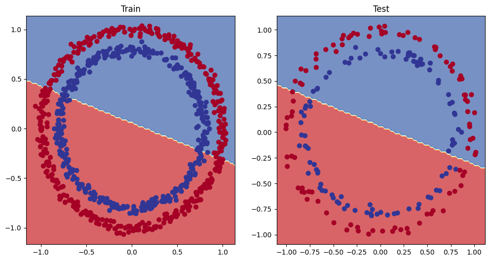
4. Make predictions and evaluate the model
From the metrics it looks like our model isn’t learning anything…
So to inspect it let’s make some predictions and make them visual!
In other words, “Visualize, visualize, visualize!”
To do so, we’re going to import a function called plot_decision_boundary() - https://github.com/mrdbourke/pytorch-deep-learning/blob/main/helper_functions.py
import requests
from pathlib import Path

# Download helper functions from Learn PyTorch repo (if it's not already downloaded)
if Path("helper_functions.py").is_file():
  print("helper_functions.py already exists, skipping download")
else:
  print("Downloading helper_functions.py")
  request = requests.get("https://raw.githubusercontent.com/mrdbourke/pytorch-deep-learning/refs/heads/main/helper_functions.py")
  with open("helper_functions.py", "wb") as f:
    f.write(request.content)

from helper_functions import plot_predictions, plot_decision_boundary
helper_functions.py already exists, skipping download
# Plot decision boundary of the model
plt.figure(figsize=(12, 6))
plt.subplot(1, 2, 1) # rows, cols, index
plt.title("Train")
plot_decision_boundary(model_0, X_train, y_train)
plt.subplot(1, 2, 2)
plt.title("Test")
plot_decision_boundary(model_0, X_test, y_test)
5. Improving a model (from a model perspective)
- Add more layers - give the model more chances to learn about patterns in the data
- Add more hidden units - go from 5 hidden units to 10 hidden units
- Fit for longer
- Changing the activation functions
- Change the learning rate
- Change the loss function
These options are all from a model’s perspective bc they deal directly with the model, rather than the data.
And bc these options are all values we (as ML engineers and data scientists) can change, they are referred as hyperparameters.
Let’s try and improve our model by:
- Adding more hidden units: 5 -> 10
- Increase the number of layers: 2 -> 3
- Increase the number of epochs: 100 -> 1000
class CircleModelV1(nn.Module):
  def __init__(self):
    super().__init__()
    self.layer_1 = nn.Linear(in_features=2, out_features=10)
    self.layer_2 = nn.Linear(in_features=10, out_features=10)
    self.layer_3 = nn.Linear(in_features=10, out_features=1)

  def forward(self, x):
    # z = self.layer_1(x)
    # z = self.layer_2(z)
    # z = self.layer_3(z)
    return self.layer_3(self.layer_2(self.layer_1(x))) # this way of writing operations leverages speed ups where possible behind the scenes

model_1 = CircleModelV1().to(device)
model_1
CircleModelV1(
  (layer_1): Linear(in_features=2, out_features=10, bias=True)
  (layer_2): Linear(in_features=10, out_features=10, bias=True)
  (layer_3): Linear(in_features=10, out_features=1, bias=True)
)
model_1.state_dict()
OrderedDict([('layer_1.weight',
              tensor([[ 0.5406,  0.5869],
                      [-0.1657,  0.6496],
                      [-0.1549,  0.1427],
                      [-0.3443,  0.4153],
                      [ 0.6233, -0.5188],
                      [ 0.6146,  0.1323],
                      [ 0.5224,  0.0958],
                      [ 0.3410, -0.0998],
                      [ 0.5451,  0.1045],
                      [-0.3301,  0.1802]], device='cuda:0')),
             ('layer_1.bias',
              tensor([-0.3258, -0.0829, -0.2872,  0.4691, -0.5582, -0.3260, -0.1997, -0.4252,
                       0.0667, -0.6984], device='cuda:0')),
             ('layer_2.weight',
              tensor([[ 0.2856, -0.2686,  0.2441,  0.0526, -0.1027,  0.1954,  0.0493,  0.2555,
                        0.0346, -0.0997],
                      [ 0.0850, -0.0858,  0.1331,  0.2823,  0.1828, -0.1382,  0.1825,  0.0566,
                        0.1606, -0.1927],
                      [-0.3130, -0.1222, -0.2426,  0.2595,  0.0911,  0.1310,  0.1000, -0.0055,
                        0.2475, -0.2247],
                      [ 0.0199, -0.2158,  0.0975, -0.1089,  0.0969, -0.0659,  0.2623, -0.1874,
                       -0.1886, -0.1886],
                      [ 0.2844,  0.1054,  0.3043, -0.2610, -0.3137, -0.2474, -0.2127,  0.1281,
                        0.1132,  0.2628],
                      [-0.1633, -0.2156,  0.1678, -0.1278,  0.1919, -0.0750,  0.1809, -0.2457,
                       -0.1596,  0.0964],
                      [ 0.0669, -0.0806,  0.1885,  0.2150, -0.2293, -0.1688,  0.2896, -0.1067,
                       -0.1121, -0.3060],
                      [-0.1811,  0.0790, -0.0417, -0.2295,  0.0074, -0.2160, -0.2683, -0.1741,
                       -0.2768, -0.2014],
                      [ 0.3161,  0.0597,  0.0974, -0.2949, -0.2077, -0.1053,  0.0494, -0.2783,
                       -0.1363, -0.1893],
                      [ 0.0009, -0.1177, -0.0219, -0.2143, -0.2171, -0.1845, -0.1082, -0.2496,
                        0.2651, -0.0628]], device='cuda:0')),
             ('layer_2.bias',
              tensor([ 0.2721,  0.0985, -0.2678,  0.2188, -0.0870, -0.1212, -0.2625, -0.3144,
                       0.0905, -0.0691], device='cuda:0')),
             ('layer_3.weight',
              tensor([[ 0.1231, -0.2595,  0.2348, -0.2321, -0.0546,  0.0661,  0.1633,  0.2553,
                        0.2881, -0.2507]], device='cuda:0')),
             ('layer_3.bias', tensor([0.0796], device='cuda:0'))])
# Create a loss function
loss_fn = torch.nn.BCEWithLogitsLoss()

# Create an optimizer
optim = torch.optim.SGD(params=model_1.parameters(),
                        lr=0.1)
# Write a training and evaluation loop for model_1
torch.manual_seed(42)
torch.cuda.manual_seed(42)

# Train for longer
epochs = 1000

# Put data on the target device
X_train, y_train = X_train.to(device), y_train.to(device)
X_test, y_test = X_test.to(device), y_test.to(device)

for epoch in range(epochs):
  ### Training
  model_1.train()
  # 1. Forward pass
  y_logits = model_1(X_train).squeeze()
  y_pred = torch.round(torch.sigmoid(y_logits)) # logits -> pred probabilities -> prediction labels

  # 2. Calculate the loss/acc
  loss = loss_fn(y_logits, y_train)
  acc = accuracy_fn(y_true=y_train,
                    y_pred=y_pred)

  # 3. Optimizer zero grad
  optimizer.zero_grad()

  # 4. Loss backward (backpropagation)
  loss.backward()

  # 5. Optimizer setp (gradient descent)
  optimizer.step()

  ### Testing
  model_1.eval()
  with torch.inference_mode():
    # 1. Forward pass
    test_logits = model_1(X_test).squeeze()
    test_pred = torch.round(torch.sigmoid(test_logits))
    # 2. Calculate the loss
    test_loss = loss_fn(test_logits,
                        y_test)
    test_acc = accuracy_fn(y_true=y_test,
                           y_pred=test_pred)

  # Print out what's happening
  if epoch % 100 == 0:
    print(f"Epoch: {epoch} | Loss: {loss:.5f}, Acc: {acc:.2f}% | Test loss: {test_loss:.5f}, Test acc: {test_acc:.2f}%")
Epoch: 0 | Loss: 0.69396, Acc: 50.88% | Test loss: 0.69261, Test acc: 51.00%
Epoch: 100 | Loss: 0.69396, Acc: 50.88% | Test loss: 0.69261, Test acc: 51.00%
Epoch: 200 | Loss: 0.69396, Acc: 50.88% | Test loss: 0.69261, Test acc: 51.00%
Epoch: 300 | Loss: 0.69396, Acc: 50.88% | Test loss: 0.69261, Test acc: 51.00%
Epoch: 400 | Loss: 0.69396, Acc: 50.88% | Test loss: 0.69261, Test acc: 51.00%
Epoch: 500 | Loss: 0.69396, Acc: 50.88% | Test loss: 0.69261, Test acc: 51.00%
Epoch: 600 | Loss: 0.69396, Acc: 50.88% | Test loss: 0.69261, Test acc: 51.00%
Epoch: 700 | Loss: 0.69396, Acc: 50.88% | Test loss: 0.69261, Test acc: 51.00%
Epoch: 800 | Loss: 0.69396, Acc: 50.88% | Test loss: 0.69261, Test acc: 51.00%
Epoch: 900 | Loss: 0.69396, Acc: 50.88% | Test loss: 0.69261, Test acc: 51.00%
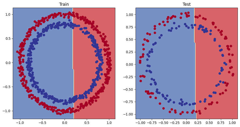
# Plot decision boundary of the model
plt.figure(figsize=(12, 6))
plt.subplot(1, 2, 1) # rows, cols, index
plt.title("Train")
plot_decision_boundary(model_1, X_train, y_train)
plt.subplot(1, 2, 2)
plt.title("Test")
plot_decision_boundary(model_1, X_test, y_test)
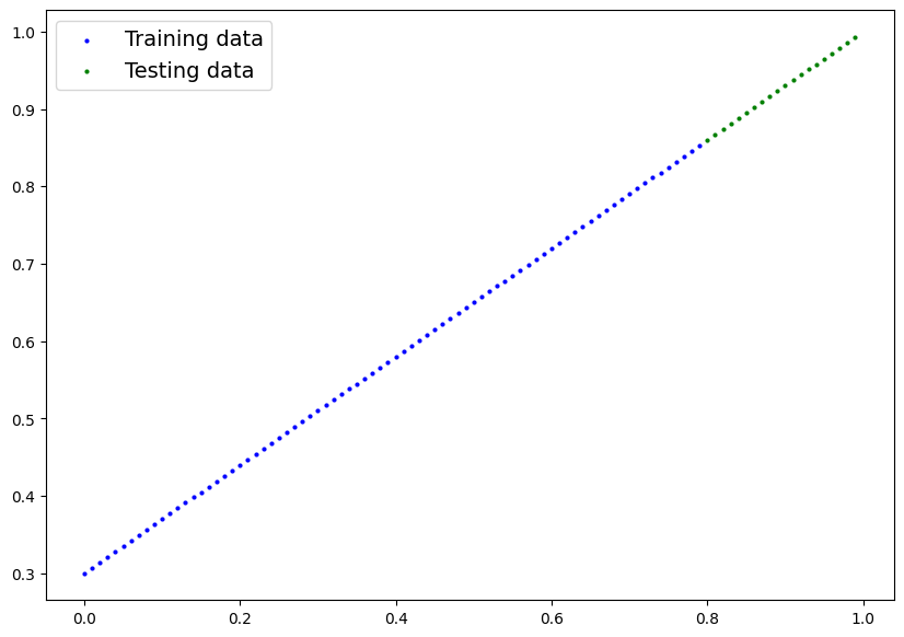
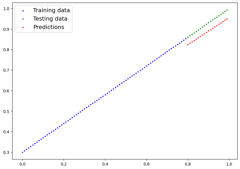
5.1 Preparing data to see if our model can fit a straight line
One way to troubleshoot to a larger problem is to test out a smaller problem.
# Create some data (same as notebook 01)
weight = 0.7
bias = 0.3
start = 0
end = 1
step = 0.01

# Create data
X_regression = torch.arange(start, end, step).unsqueeze(dim=1)
y_regression = weight * X_regression + bias # Linear regression formula (without epsilon)

# Check the data
print(len(X_regression))
X_regression[:5], y_regression[:5]
100


(tensor([[0.0000],
         [0.0100],
         [0.0200],
         [0.0300],
         [0.0400]]),
 tensor([[0.3000],
         [0.3070],
         [0.3140],
         [0.3210],
         [0.3280]]))
# Create train and test splits
train_split = int(0.8 * len(X_regression))
X_train_regression, y_train_regression = X_regression[:train_split], y_regression[:train_split]
X_test_regression, y_test_regression = X_regression[train_split:], y_regression[train_split:]

# Check the lengths of each
len(X_train_regression), len(X_test_regression), len(y_train_regression), len(y_test_regression)
(80, 20, 80, 20)
plot_predictions(train_data=X_train_regression,
                 train_labels=y_train_regression,
                 test_data=X_test_regression,
                 test_labels=y_test_regression);
X_train_regression[:10], y_train_regression[:10] # we have one feature per one label now!
(tensor([[0.0000],
         [0.0100],
         [0.0200],
         [0.0300],
         [0.0400],
         [0.0500],
         [0.0600],
         [0.0700],
         [0.0800],
         [0.0900]]),
 tensor([[0.3000],
         [0.3070],
         [0.3140],
         [0.3210],
         [0.3280],
         [0.3350],
         [0.3420],
         [0.3490],
         [0.3560],
         [0.3630]]))
5.2 Adjusting model_1 to fit a straight line
# Same architecture as model_1 (but using nn.Sequential())
model_2 = nn.Sequential(
    nn.Linear(in_features=1, out_features=10),
    nn.Linear(in_features=10, out_features=10),
    nn.Linear(in_features=10, out_features=1)
).to(device)

model_2
Sequential(
  (0): Linear(in_features=1, out_features=10, bias=True)
  (1): Linear(in_features=10, out_features=10, bias=True)
  (2): Linear(in_features=10, out_features=1, bias=True)
)
# Loss and optimizer
loss_fn = nn.L1Loss() # bc we are dealing with a regression problem, instead of a classification problem # MAE loss with regression data
optimizer = torch.optim.SGD(params=model_2.parameters(),
                            lr=0.01)
# Train the model
torch.manual_seed(42)
torch.cuda.manual_seed(42)

# Set the number of epochs
epochs = 1000

# Put the data on the target device
X_train_regression, y_train_regression = X_train_regression.to(device), y_train_regression.to(device)
X_test_regression, y_test_regression = X_test_regression.to(device), y_test_regression.to(device)

# Training
for epoch in range(epochs):
  y_pred = model_2(X_train_regression)
  loss = loss_fn(y_pred, y_train_regression)
  optimizer.zero_grad()
  loss.backward()
  optimizer.step()

  # Testing
  model_2.eval()
  with torch.inference_mode():
    test_pred = model_2(X_test_regression)
    test_loss = loss_fn(test_pred, y_test_regression)

  # Print out what's happening
  if epoch % 100 == 0:
    print(f"Epoch: {epoch} | Loss: {loss:.5f} | Test loss: {test_loss:.5f}")
Epoch: 0 | Loss: 0.75986 | Test loss: 0.91103
Epoch: 100 | Loss: 0.02858 | Test loss: 0.00081
Epoch: 200 | Loss: 0.02533 | Test loss: 0.00209
Epoch: 300 | Loss: 0.02137 | Test loss: 0.00305
Epoch: 400 | Loss: 0.01964 | Test loss: 0.00341
Epoch: 500 | Loss: 0.01940 | Test loss: 0.00387
Epoch: 600 | Loss: 0.01903 | Test loss: 0.00379
Epoch: 700 | Loss: 0.01878 | Test loss: 0.00381
Epoch: 800 | Loss: 0.01840 | Test loss: 0.00329
Epoch: 900 | Loss: 0.01798 | Test loss: 0.00360
# Turn on evaluation mode
model_2.eval()

# Make predictions (inference)
with torch.inference_mode():
  y_preds = model_2(X_test_regression)

# Plot data and predictions
plot_predictions(train_data=X_train_regression.cpu(),
                 train_labels=y_train_regression.cpu(),
                 test_data=X_test_regression.cpu(),
                 test_labels=y_test_regression.cpu(),
                 predictions=y_preds.cpu());
6. The missing piece: non-linearity
“What patterns could you draw if you were given an infinite amount of straight and non-straight lines?”
Or in ML terms, an infinite (but really it is finite) of linear and non-linear functions?
6.1 Recreating non-linear data (red and blue circles)
# Make and plot data
import matplotlib.pyplot as plt
from sklearn.datasets import make_circles

n_samples = 1000

X, y = make_circles(n_samples,
                    noise=0.03,
                    random_state=42)

plt.scatter(X[:, 0], X[:, 1], c=y, cmap=plt.cm.RdYlBu);

# Convert data to tensors and then to train and test splits
import torch
from sklearn.model_selection import train_test_split

# Turn data into tensors
X = torch.from_numpy(X).type(torch.float)
y = torch.from_numpy(y).type(torch.float)

# Split into train and test sets
X_train, X_teset, y_train, y_test = train_test_split(X,
                                                     y,
                                                     test_size=0.2,
                                                     random_state=42)

X_train[:5], y_train[:5]
(tensor([[ 0.6579, -0.4651],
         [ 0.6319, -0.7347],
         [-1.0086, -0.1240],
         [-0.9666, -0.2256],
         [-0.1666,  0.7994]]),
 tensor([1., 0., 0., 0., 1.]))
6.2 Building a model with non-linearity
- Linear = straight line
- Non-linear = non-straight line
Artificial neural networks are a large combination of linear (straight) and non-straight (non-linear) functions which are potentially able to find patterns in data.
# Build a model with non-linear activation functions
from torch import nn
class CircleModelV2(nn.Module):
  def __init__(self):
    super().__init__()
    self.layer_1 = nn.Linear(in_features=2, out_features=10)
    self.layer_2 = nn.Linear(in_features=10, out_features=10)
    self.layer_3 = nn.Linear(in_features=10, out_features=1)
    self.relu = nn.ReLU() # relu is a non-linear activation function, turns neg values to 0 and leaves pos values

  def forward(self, x):
    # Were should we put our non-linear activation functions?
    return self.layer_3(self.relu(self.layer_2(self.relu(self.layer_1(x)))))

model_3 = CircleModelV2().to(device)
model_3
CircleModelV2(
  (layer_1): Linear(in_features=2, out_features=10, bias=True)
  (layer_2): Linear(in_features=10, out_features=10, bias=True)
  (layer_3): Linear(in_features=10, out_features=1, bias=True)
  (relu): ReLU()
)
# Setup loss and optimizer
loss_fn = nn.BCEWithLogitsLoss()
optimizer = torch.optim.SGD(params=model_3.parameters(),
                            lr=1.0)
6.3 Training a model with non-linearity
# Random seeds
torch.manual_seed(42)
torch.cuda.manual_seed(42)

# Put all data on target device
X_train, y_train = X_train.to(device), y_train.to(device)
X_test, y_test = X_test.to(device), y_test.to(device)

# Loop through data
epochs = 1000

for epoch in range(epochs):
  ### Training
  model_3.train()

  # 1. Forward pass
  y_logits = model_3(X_train).squeeze()
  y_pred = torch.round(torch.sigmoid(y_logits)) # logits -> prediction probabilities -> prediction labels

  # 2. Calculate the loss
  loss = loss_fn(y_logits, y_train) # BCEWithLogitsLoss (takes in logits as first input)
  acc = accuracy_fn(y_true=y_train,
                    y_pred=y_pred)

  # 3. Optimizer zero grad
  optimizer.zero_grad()

  # 4. Loss backward
  loss.backward()

  # 5. Optimizer step
  optimizer.step()

  ### Testing
  model_3.eval()
  with torch.inference_mode():
    test_logits = model_3(X_test).squeeze()
    test_pred = torch.round(torch.sigmoid(test_logits))

    test_loss = loss_fn(test_logits, y_test)
    test_acc = accuracy_fn(y_true=y_test,
                           y_pred=test_pred)

  # Print out what's happening
  if epoch % 100 == 0:
    print(f"Epoch: {epoch} | Loss: {loss:.4f}, Acc: {acc:.2f}% | Test loss: {test_loss:.4f}, Test Acc: {test_acc:.2f}%")
Epoch: 0 | Loss: 0.6929, Acc: 50.00% | Test loss: 0.6926, Test Acc: 50.00%
Epoch: 100 | Loss: 0.5772, Acc: 86.38% | Test loss: 0.5762, Test Acc: 86.50%
Epoch: 200 | Loss: 1.4209, Acc: 50.00% | Test loss: 0.5730, Test Acc: 62.50%
Epoch: 300 | Loss: 0.2256, Acc: 97.38% | Test loss: 0.2157, Test Acc: 97.00%
Epoch: 400 | Loss: 0.0256, Acc: 100.00% | Test loss: 0.0445, Test Acc: 100.00%
Epoch: 500 | Loss: 0.0093, Acc: 100.00% | Test loss: 0.0244, Test Acc: 100.00%
Epoch: 600 | Loss: 0.0056, Acc: 100.00% | Test loss: 0.0174, Test Acc: 100.00%
Epoch: 700 | Loss: 0.0039, Acc: 100.00% | Test loss: 0.0142, Test Acc: 100.00%
Epoch: 800 | Loss: 0.0030, Acc: 100.00% | Test loss: 0.0124, Test Acc: 100.00%
Epoch: 900 | Loss: 0.0025, Acc: 100.00% | Test loss: 0.0112, Test Acc: 100.00%
6.4 Evaluating a model trained with non-linear activation functions
# Make predictions
model_3.eval()
with torch.inference_mode():
  y_preds = torch.round(torch.sigmoid(model_3(X_test))).squeeze()
y_preds[:10],  y_test[:10]
(tensor([1., 0., 1., 0., 1., 1., 0., 0., 1., 0.], device='cuda:0'),
 tensor([1., 0., 1., 0., 1., 1., 0., 0., 1., 0.], device='cuda:0'))
# Plot decision boundaries
plt.figure(figsize=(12, 6))
plt.subplot(1, 2, 1)
plt.title("Train")
plot_decision_boundary(model_1, X_train, y_train) # model_1 = no non-linearity
plt.subplot(1, 2, 2)
plt.title("Test")
plot_decision_boundary(model_3, X_test, y_test) # model_3 = non-linearity
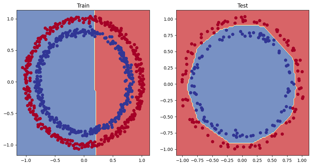
Challenge: Improve the model_3 to do better than 80% accuracy on the test data
Solution: Solved by adjusting the learning rate to lr = 1.0
7. Replicating non-linear activation functions
Neural networks, rather than telling the model what to learn, we give it the tools to discover patterns in data and it tries to figure out the patterns on its own.
And these tools are linear & non-linear functions.
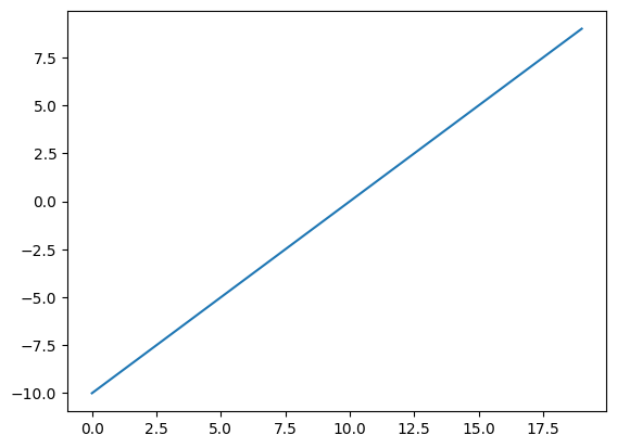
# Create a tensor
A = torch.arange(-10, 10, 1, dtype=torch.float32)
A.dtype
torch.float32
A
tensor([-10.,  -9.,  -8.,  -7.,  -6.,  -5.,  -4.,  -3.,  -2.,  -1.,   0.,   1.,
          2.,   3.,   4.,   5.,   6.,   7.,   8.,   9.])
# Visualize the tensor
plt.plot(A);
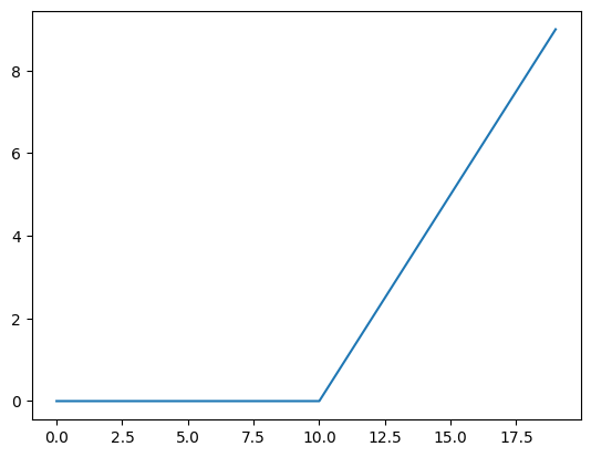
plt.plot(torch.relu(A));

def relu(x: torch.Tensor) -> torch.Tensor:
  return torch.maximum(torch.tensor(0), x) # inputs must be tensors

relu(A)
tensor([0., 0., 0., 0., 0., 0., 0., 0., 0., 0., 0., 1., 2., 3., 4., 5., 6., 7.,
        8., 9.])
# Plot ReLU activation function
plt.plot(relu(A));
# Now let's do the same for sigmoid - https://pytorch.org/docs/stable/generated/torch.nn.Sigmoid.html
def sigmoid(x: torch.Tensor):
  return 1 / (1 + torch.exp(-x))
plt.plot(torch.sigmoid(A));
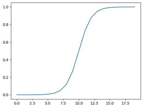
plt.plot(sigmoid(A));

8. Putting it all together with a multi-class classification problem
- Binary classification = one thing or another (cat vs. dog, spam vs. not spam, fraud or not fraud)
- Multi-class classification = more than one thing or another (cat vs. dog vs. chicken)
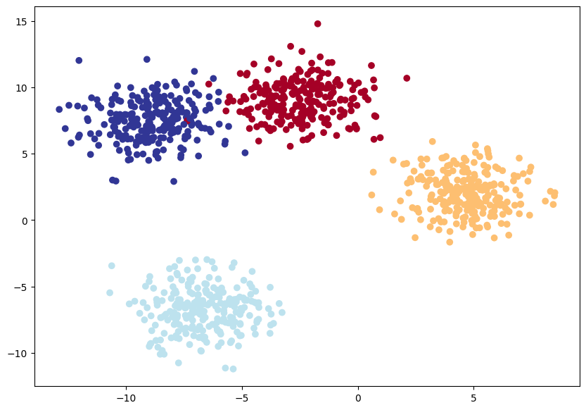
8.1 Creating a toy multi-class dataset
# Import dependencies
import torch
import matplotlib.pyplot as plt
from sklearn.datasets import make_blobs # https://scikit-learn.org/1.5/modules/generated/sklearn.datasets.make_blobs.html
from sklearn.model_selection import train_test_split

# Set the hyperparameters for data creation (often in capital letters)
NUM_CLASSES = 4
NUM_FEATURES = 2
RANDOM_SEED = 42

# 1. Create multi-class data
X_blob, y_blob = make_blobs(n_samples=1000,
                            n_features=NUM_FEATURES,
                            centers=NUM_CLASSES,
                            cluster_std=1.5, # give the clusters a little shake up
                            random_state=RANDOM_SEED)

# 2. Turn data into tensors
X_blob = torch.from_numpy(X_blob).type(torch.float)
y_blob = torch.from_numpy(y_blob).type(torch.LongTensor)

# 3. Split into train and test
X_blob_train, X_blob_test, y_blob_train, y_blob_test = train_test_split(X_blob,
                                                                        y_blob,
                                                                        test_size=0.2,
                                                                        random_state=RANDOM_SEED)

# 4. Plot data (visualize, visualize, visualize)
plt.figure(figsize=(10, 7))
plt.scatter(X_blob[:, 0], X_blob[:, 1], c=y_blob, cmap=plt.cm.RdYlBu);
8.2 Building a multi-class classification model in PyTorch
# Create device agnostic code
device = "cuda" if torch.cuda.is_available() else "cpu"
device
'cuda'
# Build a multi-class classification model
class BlobModel(nn.Module):
  def __init__(self, input_features, output_features, hidden_units=8):
    """Initializes multi-class classification model.

    Args:
      input_features (int): Number of input features to the model
      output_features (int): Number of output features (number of output classes)
      hidden_units (int): Number of hidden units between layers, default 8

    Returns: model with the specified features

    Example: -
    """
    super().__init__()
    self.linear_layer_stack = nn.Sequential(
        nn.Linear(in_features=input_features, out_features=hidden_units),
        nn.ReLU(),
        nn.Linear(in_features=hidden_units, out_features=hidden_units),
        nn.ReLU(),
        nn.Linear(in_features=hidden_units, out_features=output_features)
    )

  def forward(self, x):
    return self.linear_layer_stack(x)

# Create an instance of BlobModel and send it to the target device
model_4 = BlobModel(input_features=2,
                    output_features=4,
                    hidden_units=8).to(device)

model_4
BlobModel(
  (linear_layer_stack): Sequential(
    (0): Linear(in_features=2, out_features=8, bias=True)
    (1): ReLU()
    (2): Linear(in_features=8, out_features=8, bias=True)
    (3): ReLU()
    (4): Linear(in_features=8, out_features=4, bias=True)
  )
)
X_blob_train.shape, y_blob_train[:5]
(torch.Size([800, 2]), tensor([1, 0, 2, 2, 0]))
torch.unique(y_blob_train) # shows the classes
tensor([0, 1, 2, 3])
8.3 Create a loss function and an optimizer for a multi-class classification model
# Create a loss function for multi-class classification - loss function measures how wrong our model's prediction are
loss_fn = nn.CrossEntropyLoss()

# Create an optimizer for multi-class classification - optimizer updates our model parameters to try and reduce the loss
optimizer = torch.optim.SGD(params=model_4.parameters(),
                            lr=0.1) # learning rate is a hyperparamete you can change
8.4 Getting prediction probabilities for a multi-class PyTorch model
In order to evaluate and train and test our model, we need to convert our model’s outputs (logits) to prediction probabilities and then to prediction labels.
Logits (raw output of the model) -> Pred probs (use torch.softmax) -> Pred labels (take the argmax of the prediction probabilities)
# Lets's get some raw outputs of our model (logits)
model_4.eval()
with torch.inference_mode():
  y_logits = model_4(X_blob_test.to(device))

y_logits[:10]
tensor([[-0.7646, -0.7412, -1.5777, -1.1376],
        [-0.0973, -0.9431, -0.5963, -0.1371],
        [ 0.2528, -0.2379,  0.1882, -0.0066],
        [-0.4134, -0.5204, -0.9303, -0.6963],
        [-0.3118, -1.3736, -1.1991, -0.3834],
        [-0.1497, -1.0617, -0.7107, -0.1645],
        [ 0.1539, -0.2887,  0.1520, -0.0109],
        [-0.2154, -1.1795, -0.9300, -0.2745],
        [ 0.2443, -0.2472,  0.1649,  0.0061],
        [-0.2329, -1.2120, -0.9849, -0.3004]], device='cuda:0')
y_blob_test[:10]
tensor([1, 3, 2, 1, 0, 3, 2, 0, 2, 0])
# Convert our model's logit outputs to prediction probabilities
y_pred_probs = torch.softmax(y_logits, dim=1)
print(y_logits[:5])
print(y_pred_probs[:5])
tensor([[-0.7646, -0.7412, -1.5777, -1.1376],
        [-0.0973, -0.9431, -0.5963, -0.1371],
        [ 0.2528, -0.2379,  0.1882, -0.0066],
        [-0.4134, -0.5204, -0.9303, -0.6963],
        [-0.3118, -1.3736, -1.1991, -0.3834]], device='cuda:0')
tensor([[0.3169, 0.3244, 0.1405, 0.2182],
        [0.3336, 0.1432, 0.2026, 0.3206],
        [0.3011, 0.1843, 0.2823, 0.2323],
        [0.3078, 0.2766, 0.1836, 0.2320],
        [0.3719, 0.1286, 0.1532, 0.3463]], device='cuda:0')
torch.sum(y_pred_probs[0])
tensor(1., device='cuda:0')
torch.argmax(y_pred_probs[0]) # for sample 0, class 1 is the right class
tensor(1, device='cuda:0')
# Convert our model's prediction probabilities to prediction labels
y_preds = torch.argmax(y_pred_probs, dim=1)
y_preds
tensor([1, 0, 0, 0, 0, 0, 0, 0, 0, 0, 0, 1, 0, 0, 0, 0, 0, 0, 0, 0, 0, 0, 0, 0,
        0, 0, 0, 0, 0, 0, 0, 1, 0, 0, 1, 0, 0, 0, 0, 0, 0, 0, 0, 0, 0, 0, 0, 0,
        0, 3, 0, 0, 0, 0, 0, 0, 0, 1, 0, 0, 0, 0, 0, 0, 0, 0, 0, 0, 0, 0, 0, 0,
        0, 0, 0, 0, 0, 0, 0, 0, 0, 0, 0, 0, 0, 0, 0, 0, 0, 0, 0, 0, 1, 0, 0, 0,
        1, 0, 0, 0, 0, 0, 0, 0, 0, 0, 0, 0, 0, 0, 0, 0, 0, 0, 0, 0, 0, 0, 0, 0,
        0, 0, 0, 0, 0, 0, 0, 0, 0, 0, 0, 0, 0, 0, 0, 3, 0, 0, 1, 0, 1, 0, 0, 0,
        0, 0, 0, 0, 3, 0, 0, 1, 0, 0, 0, 0, 0, 0, 0, 1, 0, 0, 0, 0, 0, 0, 0, 0,
        0, 0, 0, 0, 0, 1, 1, 1, 0, 0, 0, 1, 0, 0, 0, 1, 0, 0, 0, 0, 0, 0, 0, 0,
        1, 0, 0, 0, 0, 1, 0, 1], device='cuda:0')
y_blob_test
tensor([1, 3, 2, 1, 0, 3, 2, 0, 2, 0, 0, 1, 0, 0, 0, 3, 3, 2, 3, 3, 3, 0, 1, 2,
        2, 2, 3, 0, 1, 0, 3, 1, 1, 3, 1, 2, 1, 3, 0, 2, 0, 3, 3, 2, 0, 3, 1, 1,
        0, 3, 1, 0, 1, 1, 3, 2, 1, 1, 3, 2, 2, 0, 3, 2, 2, 0, 0, 3, 3, 0, 0, 3,
        3, 3, 2, 3, 3, 3, 3, 1, 0, 2, 3, 2, 3, 3, 2, 3, 3, 2, 3, 3, 1, 3, 3, 3,
        1, 0, 3, 2, 0, 0, 3, 0, 2, 3, 1, 0, 3, 2, 1, 1, 0, 2, 2, 3, 0, 0, 1, 2,
        2, 3, 0, 1, 2, 0, 0, 0, 2, 3, 1, 2, 3, 2, 0, 3, 0, 0, 1, 1, 1, 0, 2, 2,
        2, 2, 0, 3, 3, 2, 2, 1, 3, 2, 0, 0, 3, 3, 2, 1, 2, 0, 3, 2, 0, 3, 2, 0,
        2, 2, 2, 0, 3, 1, 1, 1, 1, 1, 3, 1, 0, 2, 2, 1, 2, 2, 0, 1, 2, 2, 0, 0,
        1, 3, 2, 0, 3, 1, 2, 1])
8.5 Create a training loop and testing loop for a multi-class PyTorch model
# Fit the multi-class model to the data
torch.manual_seed(42)
torch.cuda.manual_seed(42)

# Set number of epochs
epochs = 100

# Put data to target device
X_blob_train, y_blob_train = X_blob_train.to(device), y_blob_train.to(device)
X_blob_test, y_blob_test = X_blob_test.to(device), y_blob_test.to(device)

# Loop through data
for epoch in range(epochs):
  ### Training
  model_4.train()

  y_logits = model_4(X_blob_train).squeeze()
  y_pred = torch.softmax(y_logits, dim=1).argmax(dim=1)

  loss = loss_fn(y_logits, y_blob_train)
  acc = accuracy_fn(y_true=y_blob_train,
                    y_pred=y_pred)

  optimizer.zero_grad()
  loss.backward()
  optimizer.step()

  ### Testing
  model_4.eval()
  with torch.inference_mode():
    test_logits = model_4(X_blob_test).squeeze()
    test_preds = torch.softmax(test_logits, dim=1).argmax(dim=1)

    test_loss = loss_fn(test_logits, y_blob_test)
    test_acc = accuracy_fn(y_true=y_blob_test,
                           y_pred=test_preds)

  # Print out what's happening
  if epoch % 10 == 0:
    print(f"Epoch: {epoch} | Loss: {loss:.4f}, Acc: {acc:.2f}% | Test loss: {test_loss:.4f}, Test Acc: {test_acc:.2f}%")
Epoch: 0 | Loss: 1.1588, Acc: 40.38% | Test loss: 1.0755, Test Acc: 48.00%
Epoch: 10 | Loss: 0.6448, Acc: 96.75% | Test loss: 0.6607, Test Acc: 97.50%
Epoch: 20 | Loss: 0.4254, Acc: 98.50% | Test loss: 0.4307, Test Acc: 100.00%
Epoch: 30 | Loss: 0.2529, Acc: 99.12% | Test loss: 0.2451, Test Acc: 99.50%
Epoch: 40 | Loss: 0.1123, Acc: 99.25% | Test loss: 0.1023, Test Acc: 99.50%
Epoch: 50 | Loss: 0.0663, Acc: 99.25% | Test loss: 0.0585, Test Acc: 99.50%
Epoch: 60 | Loss: 0.0507, Acc: 99.25% | Test loss: 0.0429, Test Acc: 99.50%
Epoch: 70 | Loss: 0.0430, Acc: 99.25% | Test loss: 0.0349, Test Acc: 99.50%
Epoch: 80 | Loss: 0.0384, Acc: 99.25% | Test loss: 0.0299, Test Acc: 99.50%
Epoch: 90 | Loss: 0.0352, Acc: 99.25% | Test loss: 0.0266, Test Acc: 99.50%
8.6 Making and evaluating predictions with a PyTorch multi-class model
# Make predictions
model_4.eval()
with torch.inference_mode():
  y_logits = model_4(X_blob_test)

# View the first 10 predictions
y_logits[:10]
tensor([[-0.6249,  5.9860, -7.6323, -8.4470],
        [-2.1738, -6.3750, -3.7202,  3.1203],
        [-3.4102, -3.8958,  3.1567, -2.6119],
        [-1.1505,  4.1962, -3.8472, -4.8820],
        [ 3.7548, -1.3391, -9.1422, -6.9466],
        [-2.8211, -7.5767, -4.2944,  3.7944],
        [-3.0306, -3.3328,  2.7955, -2.1374],
        [ 3.3761, -4.0375, -6.8987, -3.5503],
        [-4.3620, -4.9904,  3.8123, -3.3814],
        [ 3.5012, -3.0281, -7.5401, -4.7064]], device='cuda:0')
# Go from logits -> Prediction probabilities
y_pred_probs = torch.softmax(y_logits, dim=1)
y_pred_probs[:10]
tensor([[1.3438e-03, 9.9865e-01, 1.2164e-06, 5.3854e-07],
        [4.9905e-03, 7.4740e-05, 1.0630e-03, 9.9387e-01],
        [1.3985e-03, 8.6060e-04, 9.9463e-01, 3.1073e-03],
        [4.7389e-03, 9.9483e-01, 3.1956e-04, 1.1353e-04],
        [9.9388e-01, 6.0966e-03, 2.4904e-06, 2.2378e-05],
        [1.3372e-03, 1.1504e-05, 3.0644e-04, 9.9834e-01],
        [2.9138e-03, 2.1537e-03, 9.8781e-01, 7.1181e-03],
        [9.9838e-01, 6.0198e-04, 3.4435e-05, 9.7989e-04],
        [2.8147e-04, 1.5016e-04, 9.9882e-01, 7.5044e-04],
        [9.9825e-01, 1.4575e-03, 1.5998e-05, 2.7210e-04]], device='cuda:0')
# Go from pred probs to pred labels
y_preds = torch.argmax(y_pred_probs, dim=1)
y_preds[:10]
tensor([1, 3, 2, 1, 0, 3, 2, 0, 2, 0], device='cuda:0')
plt.figure(figsize=(12, 6))
plt.subplot(1, 2, 1)
plt.title("Train")
plot_decision_boundary(model_4, X_blob_train, y_blob_train)
plt.subplot(1, 2, 2)
plt.title("Test")
plot_decision_boundary(model_4, X_blob_test, y_blob_test)
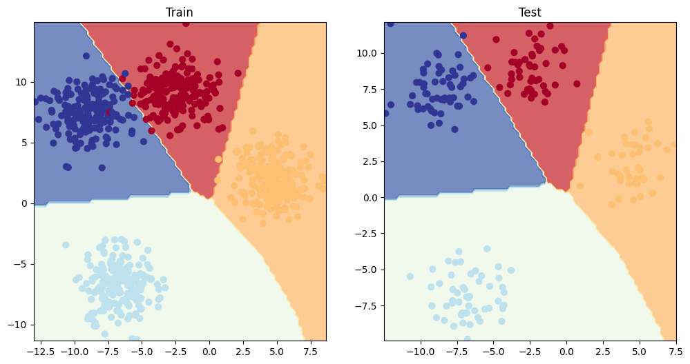
The model can also work pretty good without the ReLU layers, bc the data is linearly separable.
9. A few more classification metrics… (to evaluate our classification model)
- Accuracy - out of 100 samples, how many does our model get right?
- Precision
- Recall
- F1-score
- Confusion matrix
- Classification report
See this article for when to use precision and recall - https://towardsdatascience.com/beyond-accuracy-precision-and-recall-3da06bea9f6c
If you want access to a lot of PyTorch metrics, see TorchMetrics - https://lightning.ai/docs/torchmetrics/stable/
!pip install torchmetrics
Requirement already satisfied: torchmetrics in /usr/local/lib/python3.10/dist-packages (1.6.1)
Requirement already satisfied: numpy>1.20.0 in /usr/local/lib/python3.10/dist-packages (from torchmetrics) (1.26.4)
Requirement already satisfied: packaging>17.1 in /usr/local/lib/python3.10/dist-packages (from torchmetrics) (24.2)
Requirement already satisfied: torch>=2.0.0 in /usr/local/lib/python3.10/dist-packages (from torchmetrics) (2.5.1+cu121)
Requirement already satisfied: lightning-utilities>=0.8.0 in /usr/local/lib/python3.10/dist-packages (from torchmetrics) (0.11.9)
Requirement already satisfied: setuptools in /usr/local/lib/python3.10/dist-packages (from lightning-utilities>=0.8.0->torchmetrics) (75.1.0)
Requirement already satisfied: typing-extensions in /usr/local/lib/python3.10/dist-packages (from lightning-utilities>=0.8.0->torchmetrics) (4.12.2)
Requirement already satisfied: filelock in /usr/local/lib/python3.10/dist-packages (from torch>=2.0.0->torchmetrics) (3.16.1)
Requirement already satisfied: networkx in /usr/local/lib/python3.10/dist-packages (from torch>=2.0.0->torchmetrics) (3.4.2)
Requirement already satisfied: jinja2 in /usr/local/lib/python3.10/dist-packages (from torch>=2.0.0->torchmetrics) (3.1.4)
Requirement already satisfied: fsspec in /usr/local/lib/python3.10/dist-packages (from torch>=2.0.0->torchmetrics) (2024.10.0)
Requirement already satisfied: sympy==1.13.1 in /usr/local/lib/python3.10/dist-packages (from torch>=2.0.0->torchmetrics) (1.13.1)
Requirement already satisfied: mpmath<1.4,>=1.1.0 in /usr/local/lib/python3.10/dist-packages (from sympy==1.13.1->torch>=2.0.0->torchmetrics) (1.3.0)
Requirement already satisfied: MarkupSafe>=2.0 in /usr/local/lib/python3.10/dist-packages (from jinja2->torch>=2.0.0->torchmetrics) (3.0.2)
from torchmetrics import Accuracy

# Setup metric
torchmetric_accuracy = Accuracy(task="multiclass", num_classes=4).to(device)

# Calculate accuracy
torchmetric_accuracy(y_preds, y_blob_test)
tensor(0.9950, device='cuda:0')